A liquidity pool makes assets available under a set of trading rules. A smart order router studies those rules and available balances to estimate how a requested swap could be executed. The relationship becomes clearer when you stop thinking of a pool as a price label and start thinking of it as a function: give it a particular input, and it produces a particular output under its current conditions.
That output usually does not scale in a straight line with the input. A quote for ten tokens cannot simply be multiplied by one hundred to predict a quote for one thousand. Trade size changes how much of the available liquidity is used, which is why routing needs to consider the actual amount being exchanged.
Pool balances and executable depth
In a simple two-token pool, reserves represent amounts of the two assets held by the pool. A pricing rule connects those reserves. As a swap adds one asset and removes the other, the relationship changes, affecting the price available for subsequent amounts.
“Depth” describes how much can be exchanged at or near relevant prices. Total value locked is a broader measure and does not directly answer that question. A large amount of capital can be distributed in ways that are not useful for a particular trade, and a modest pool may have substantial depth within a narrow price interval.
The DeFi glossary distinguishes liquidity, price impact, and slippage. Keeping those terms separate makes it easier to understand why a route changes as the requested amount grows.
A hypothetical constant-product calculation
Consider an intentionally simplified pool containing 10,000 units of A and 10,000 units of B. Ignore trading fees, network costs, token transfer behavior, and rounding. Assume the pool follows the constant-product relationship x × y = k, where x and y are the reserves.
Initially, the product is 100,000,000. Adding 1,000 A brings the A reserve to 11,000. To preserve the product, the B reserve becomes 100,000,000 divided by 11,000, or approximately 9,090.91. The amount removed is therefore approximately 909.09 B.
- Starting reserves: 10,000 A and 10,000 B.
- Input: 1,000 A.
- New A reserve: 11,000 A.
- New B reserve: approximately 9,090.91 B.
- Output: approximately 909.09 B.
The initial reserve ratio was one to one, yet the swap did not return 1,000 B. The trade moved through a pricing curve. Its average execution rate differs from the starting marginal rate because each additional unit is exchanged under a progressively changed reserve balance.
This arithmetic illustrates price impact within the model. It is not a real token quote, a prediction of market value, or a formula covering every AMM design. Production pools include fees and implementation details that must be included in executable calculations.
What changes when a second pool is available?
Now introduce a second, independent hypothetical pool with the same starting reserves and rule. Split the same 1,000 A order equally, sending 500 A to each pool. Each pool’s new B reserve is 100,000,000 divided by 10,500, approximately 9,523.81. Each therefore returns approximately 476.19 B.
The combined output is approximately 952.38 B. That exceeds the 909.09 B from placing the entire order in just one pool. The example adds a second source of accessible liquidity; it does not prove that dividing an order creates value from nothing.
If both supposed paths eventually consume the same original pool, treating them as independent would overstate the available output. Likewise, executing two sequential 500 A swaps against one unchanged pool does not reset its reserves between trades. The second swap encounters the state left by the first.
This is an essential routing principle: consider the complete plan and its shared dependencies. A set of attractive individual quotes can form an unattractive combined route when those quotes compete for the same liquidity.
Gas places a price on complexity
More branches can require more onchain work. The illustrative split above improved gross output by roughly 43.29 B before any fee. Whether it improves the economic result depends on the additional cost of executing it and the assumptions used to express that cost in comparable units.
Suppose, hypothetically, that the extra execution cost equals 50 B at the comparison price. The extra output would not cover that cost. If the extra cost instead equals 5 B, the result could be preferable under the same assumptions. A route optimizer should consider the trade-off rather than maximize branch count.
Our swap-cost overview separates transferred token amounts from network fees paid in another asset. This distinction prevents an economic estimate from being mistaken for the literal number of tokens a wallet will receive.
Concentrated liquidity changes the shape of depth
Some AMMs allow providers to make liquidity available only within chosen price ranges. The official Uniswap concentrated-liquidity documentation explains how positions participate while the price is within their range and become inactive outside it.
For routing, the consequence is that depth can change as a trade crosses range boundaries. A pool that looks deep for a small amount may offer a different execution profile for a larger amount. The router needs to estimate the whole swap across the relevant liquidity distribution, rather than extrapolate indefinitely from the first price point.
Imagine a hypothetical path with abundant liquidity close to the current price but much less beyond it. A modest order might remain within the dense interval. A larger order might move past it and become relatively expensive. A second path with less impressive initial pricing but more depth farther away could then become useful.
How a routing engine approaches the problem
A conceptual routing process starts by identifying candidate markets for the specified assets and network. It considers direct connections, permitted intermediate assets, and potential splits. It then estimates each complete candidate using its requested size, applicable fees, and execution assumptions.
The search has practical limits. Exploring every possible path and every possible allocation would be expensive, so implementations choose which candidates to evaluate and how finely to test split proportions. An advertised “best route” should therefore be understood within the provider’s available sources, constraints, and search method.
There can also be a trade-off between spending more time searching and delivering a fresher quote. For a rapidly changing state, a theoretically thorough search that arrives too late may be less useful than a sufficiently good result with clear expiry and execution bounds.
A useful learning exercise is to repeat the hypothetical pool calculation with an input of 100 A, then 2,000 A, keeping starting reserves fixed. Compare the output per unit of input rather than only the absolute output. Then repeat it after doubling both reserves. These controlled changes isolate the effect of trade size and available liquidity. They also reveal why a route selected for a small trade should be recalculated when the amount changes instead of merely scaling its earlier answer.
Liquidity providers have a different problem
A trader asks what a given input can receive. A liquidity provider asks how a position behaves as prices, fees, and inventory change. Trading fees are only one component of that outcome. Providing liquidity can underperform simply holding the underlying assets when relative prices move.
Accordingly, deep liquidity should not be read as proof that providing it is risk-free or that its providers will remain indefinitely. Deposits, withdrawals, and range changes can alter future routing possibilities. A route analysis concerns liquidity available to the particular request, not a promise about future market conditions.
Use the model without overextending it
The worked calculations establish three useful ideas: size affects output, independent liquidity sources can improve a combined route, and extra execution cost can erase that improvement. Concentrated ranges add another reason to inspect the full trade rather than rely on a headline pool value.
For a broader explanation of route shapes, continue to our routing hub. DeFiRouter.com’s examples remain educational and simulated. When reading an actual quote elsewhere, ask which pools were included, whether branches share liquidity, which costs were modeled, and how execution limits handle a changing market. Those questions connect the mathematics to a reviewable transaction.